Overview of the package
The mvpoly package is a cross-language collection of basic operations on various numeric representation of multivariate polynomials.
This is not a symbolic algebra package, by a numeric representation we mean some data-structure of floating point numbers representing the coefficients of the polynomial. For dense polynomials (those with mostly non-zero coefficients) an array is the obvious choice of a data-structure, for a sparse polynomial a dictionary stucture may give better performance.
By our choice, the number of basic operations on
multivariate polynomials is quite small: addition,
mutliplication, evaluation at point or set of points,
composition, differentiation, integration (definite and
indefinite), and we implement these operations as
object methods in subclasses of a basic class MVPoly.
We have implemented an MVPolyCube subclass
which uses numpy.ndarray for the coefficients, and
a MVPolyDict subclass which uses a
dictionary.
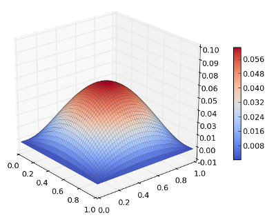
Arrays, numerics, object methods: clearly we are talking about high-level scientific environment such as Python, Matlab/Octave, Julia and the like. The basic ideas should be fairly straightforward to move between them, so far the package is ported to Python and Octave/Matlab. Python’s OO is rather slick and allows some nice syntactic sugar, for example:
import numpy as np
from mvpoly.cube import MVPolyCube

x, y = MVPolyCube.variables(2)
p = x*(1-x)*y*(1-y)

L = np.linspace(0, 1, 50)
Gx, Gy = np.meshgrid(L, L)
Gp = p(Gx, Gy)
used to generate the grid of value of the bivariate polynomial
plotted above (see the file examples/cube-eval-plot.py
included with the distribution).